Google Trend is an application of Google which shows the search terms’ trends over time for different geographies. It shows real-time search trends and daily search trends for every city in the world. Thanks to Google Trend, understanding the users’ intent through different seasons for different queries is easier. Also, real-time events and real-world entities can be noticed via Google Trend earlier. In PubMed (Medical Publication Site), there are lots of studies show that Google Trends can indicate outbreaks’ early stages to let governments take measures. Lastly, Google Trends help Google Ads and SEO campaigns to see Brand Power and related queries’ trends over time for creating a smart campaign strategy.
According to Google, thanks to Google Trends, all popular queries can be estimated with pre-search volumes with a maximum margin of 12%. While consistency was lower in entertainment and social network queries, this consistency was almost over 90% in the health, travel, and service sectors. Because of this situation, following Google Trends Data with Python in bulk can be helpful for an SEO. Also, in this article, we will learn how Google classifies search terms according to different industries and search intents so that we can clean our data even more.
What is PyTrends?
PyTrend is a Python library for using Google Trends API with Python. It allows us to produce more data faster. Also, it creates a chance to draw interactive plots for searched terms’ trend graphics over the selected time periods. Changing language, industry, geography in Pytrend is also possible. PyTrend is not an official API of Google. Also, using different time zones, extract low search volume countries, finding related queries, and rising topics are doable thanks to PyTrend.
We can start our guideline for PyTrends.
How to Install PyTrend?
The necessary code line for installing PyTrend is “pip install pytrends”. Use PyTrend to analyze the search trends with Python by installing it with the “pip” command. Type “pip install pytrends” to the “CMD Prompt”. To use PyTrends, you need to have Pandas, Requests, lxml dependencies in your Python Environment.
How to Pull Data from Google Trends via PyTrend?
To pull data from Google Trends via Python, user has to connect to the Google.
from pytrends.request import TrendReq
pytrends = TrendReq(hl='es-US', tz=360)
With these two lines of code, connecting the Google Trends is possible. “hl” stands for “Host Language” while “tz” stands for “time zone”. Google uses Central Standard Time (CST) for time management. So while using PyTrends, we need to use CST instead of Coordinated Universal Time, UTC. Using PyTrends via proxies is also possible. Since some users need to make more requests, sometimes Google Trends may block the user, the proxy is a workaround for this reason.
from pytrends.request import TrendReq
pytrends = TrendReq(hl='en-US', tz=360, timeout=(3,12), proxies=['https://192.128.156.13:80',], retries=1, backoff_factor=0.1, requests_args={'verify':False})- The timeout attribute is from the Requests Library of Python. The first argument is for “connecting”, the second one is for “read”. If a connection try lasts more than 3 seconds and a reading of the request lasts more than 12 seconds, it will give a timeout error.
- Proxies attribute is for stating the proxies which will be used for the request, the port number is obligatory.
- “Retries” is the number of retrying chances after the first failed request.
- Requests_args parameter is to comply with the nature of the request, false means ignore SSL.
- Backoff_factor is the time period between retries.
After the connection has been established, we can continue to the next section: pulling data.
How to Pull Keyword Trends with PyTrend from Google Trends
To pull data from the Google Trends, we need to determine which keywords we want to pull data about. To state that, we will create a variable below:
kw_list = ['coronavirus', 'donald trump', 'joe biden', 'china', 'elections']
pytrends.build_payload(kw_list, cat=0, timeframe='today 5-y', geo='', gprop='')- “timeframe=’today 5-y'” means 5 years from today,
- “geo” attribute is for determining the geography of the data which will be pulled from Google Trends for search trend analysis via Python programming language.
- “group” stands for Google Property which means that which vertical search you want to use such as google images, web searches or news, YouTube etc…
Thanks to these two lines of code, we can be set for pulling data for the queries in “kw_list” variable.
How to Check Interest Over Time for Given Queries in PyTrend
To check the interest over time, we need to use the method with the same name which is “interest_over_time()”. You may see the result below.
pytrends.interest_over_time()
OUTPUT>>>| coronavirus | donald trump | joe biden | china | elections | ||
|---|---|---|---|---|---|---|
| date | isPartial | |||||
| 2015-07-26 | 0 | 0 | 0 | 2 | 0 | False |
| 2015-08-02 | 0 | 1 | 0 | 2 | 0 | False |
| 2015-08-09 | 0 | 1 | 0 | 2 | 0 | False |
| 2015-08-16 | 0 | 1 | 0 | 2 | 0 | False |
| 2015-08-23 | 0 | 1 | 0 | 2 | 0 | False |
| … | … | … | … | … | … | … |
| 2020-06-14 | 13 | 1 | 0 | 3 | 0 | False |
| 2020-06-21 | 13 | 1 | 0 | 2 | 0 | False |
| 2020-06-28 | 13 | 1 | 0 | 3 | 0 | False |
| 2020-07-05 | 13 | 1 | 0 | 2 | 0 | False |
| 2020-07-12 | 13 | 1 | 0 | 2 | 0 | False |
From 5 years today, we have taken the Trends Information for the given queries. As we may see that in 2015, Coronavirus has a 0 interest over time but in 2020 it starts to increase its trend curve. Also, Donald Trump is always between 0-1 and Joe Biden is always 0. So, as you may see, there might be some misunderstanding here. Let’s check together.
First, we have used the Search Term instead of the Topic or Entity Profile, that’s why the information in the table for Political Figures are not reflected as correct. Second, we have used “0” for “cat” attribute. Google Trends classifies queries according to their search intent, and checking these trend classes can be useful to understand Google’s perception for categorization.
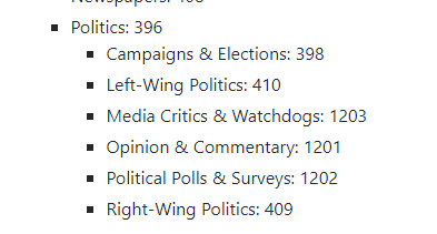
According to the Categorization, “Politics” has the number 396. If we change the categorization and timeline like below:
pytrends.build_payload(kw_list, cat=396, timeframe='today 3-m', geo='US', gprop='')| coronavirus | Donald Trump | Joe Biden | China | Elections | ||
|---|---|---|---|---|---|---|
| date | isPartial | |||||
| 2020-04-21 | 37 | 3 | 14 | 5 | 17 | False |
| 2020-04-22 | 27 | 4 | 11 | 3 | 15 | False |
| 2020-04-23 | 32 | 5 | 15 | 7 | 15 | False |
| 2020-04-24 | 28 | 7 | 14 | 5 | 15 | False |
| 2020-04-25 | 21 | 3 | 13 | 4 | 10 | False |
| … | … | … | … | … | … | … |
| 2020-07-14 | 18 | 6 | 19 | 2 | 38 | False |
| 2020-07-15 | 19 | 7 | 21 | 2 | 49 | False |
| 2020-07-16 | 13 | 5 | 19 | 3 | 23 | False |
| 2020-07-17 | 10 | 5 | 16 | 1 | 25 | False |
| 2020-07-18 | 15 | 8 | 18 | 3 | 19 | False |
In this example, we have only pulled the data for “Politic Web Searches” for the last 3 months from the United States. But still, our data is not like completely realistic. It is closer to reality than before but, still now enough. To see the reason for this, we need to use different variations for our keyword list.
First, let’s change our category back to 0 which means all categories:
pytrends.build_payload(kw_list, cat=0, timeframe='today 3-m', geo='GB')
pytrends.interest_over_time()| Coronavirus | Trump | Joe Biden | China | Elections | ||
|---|---|---|---|---|---|---|
| date | isPartial | |||||
| 2020-04-21 | 100 | 3 | 0 | 3 | 0 | False |
| 2020-04-22 | 68 | 3 | 0 | 4 | 0 | False |
| 2020-04-23 | 67 | 3 | 0 | 4 | 0 | False |
| 2020-04-24 | 93 | 14 | 0 | 3 | 0 | False |
| 2020-04-25 | 67 | 9 | 0 | 4 | 0 | False |
| … | … | … | … | … | … | … |
| 2020-07-14 | 28 | 3 | 0 | 3 | 0 | False |
| 2020-07-15 | 24 | 4 | 0 | 3 | 0 | False |
| 2020-07-16 | 24 | 4 | 0 | 3 | 0 | False |
| 2020-07-17 | 25 | 3 | 0 | 3 | 0 | False |
| 2020-07-18 | 22 | 4 | 0 | 3 | 0 | False |
Now, you may see that Coronavirus search trends is way much more realistic. It has a peak during April and in the summer months it has decreased its trend. But, still, our political figures don’t have so much attention like always do. Let’s change our keyword list this time:
kw_list = ['Donald Trump']
pytrends.build_payload(kw_list, cat=0, timeframe='today 3-m', geo='GB')| Donald Trump | ||
|---|---|---|
| date | isPartial | |
| 2020-04-21 | 21 | False |
| 2020-04-22 | 23 | False |
| 2020-04-23 | 20 | False |
| 2020-04-24 | 100 | False |
| 2020-04-25 | 62 | False |
| … | … | … |
| 2020-07-14 | 19 | False |
| 2020-07-15 | 24 | False |
| 2020-07-16 | 18 | False |
| 2020-07-17 | 18 | False |
| 2020-07-18 | 18 | False |
Data is way much more realistic. Now, we can check Donald Trump’s and Joe Biden’s trend curves at the same time.
kw_list = ['Donald Trump', 'Joe Biden']
pytrends.build_payload(kw_list, cat=0, timeframe='today 3-m', geo='GB')| Donald Trump | Joe Biden | isPartial | |
|---|---|---|---|
| date | |||
| 2020-04-21 | 21 | 2 | False |
| 2020-04-22 | 24 | 1 | False |
| 2020-04-23 | 21 | 2 | False |
| 2020-04-24 | 100 | 3 | False |
| 2020-04-25 | 58 | 4 | False |
| … | … | … | … |
| 2020-07-14 | 18 | 2 | False |
| 2020-07-15 | 24 | 2 | False |
| 2020-07-16 | 17 | 2 | False |
| 2020-07-17 | 16 | 4 | False |
| 2020-07-18 | 18 | 2 | False |
It is not realistic again, Donald Trump’s trend curve has been changed and also Joe Biden’s trend curve is so much weaker than the real. What is the reason for this? First, the “isPartial” section may catch your attention, it is not related to this situation, but it shows whether the data includes estimations or not. The real reason for this difference is that every search term and the entity has its own curve as it is, but if you unify the queries in a list, they will change their curve in a competition with a relativist way.
Let’s check Joe Biden’s trend curve just only for him:
kw_list = ['Joe Biden']
pytrends.build_payload(kw_list, cat=0, timeframe='today 3-m', geo='GB')
pytrends.interest_over_time()| Joe Biden | ||
|---|---|---|
| date | isPartial | |
| 2020-04-21 | 16 | False |
| 2020-04-22 | 10 | False |
| 2020-04-23 | 15 | False |
| 2020-04-24 | 30 | False |
| 2020-04-25 | 28 | False |
| … | … | … |
| 2020-07-14 | 19 | False |
| 2020-07-15 | 25 | False |
| 2020-07-16 | 14 | False |
| 2020-07-17 | 25 | False |
| 2020-07-18 | 22 | False |
It is way much different, because it has been calculated with only its own values.
What is the solution for this problem? How can we calculate the trend curve one by one for every query? With a for loop. You may follow the code below to perform the same process for each query one by one.
Let’s begin to our PyTrend guideline.
First, we need to create our “keyword list” which consist of our targeted search terms.
kw_list = ['Joe Biden', 'Donald Trump', 'Hillary Clinton', 'Bernie Sanders', 'Elizabeth Warren', 'Jane Sanders', 'Tulsi Gabbard', 'Barack Obama']Now, we need to create a nested list so that “build_load()” method can deal with every query one by one.
kw_group = list(zip(*[iter(kw_list)]*1))
print(kw_group)
OUTPUT>>>
[('Joe Biden',), ('Donald Trump',), ('Hillary Clinton',), ('Bernie Sanders',), ('Elizabeth Warren',), ('Jane Sanders',), ('Tulsi Gabbard',), ('Barack Obama',)]With this code, we have turned our list into a tuple collection in a list. “Iter” is being used for “iteration”, “zip” is being used for creating tuples which from the elements of different variables. In this example, since we have only one list, it has created a tuple collection only from one variable.
Now, we need to turn every tuple into a list, we will use the List Comprehension Method.
kw_grplist = [list(x) for x in kw_group]
print(kw_grplist)
OUTPUT>>>
[['Joe Biden'], ['Donald Trump'], ['Hillary Clinton'], ['Bernie Sanders'], ['Elizabeth Warren'], ['Jane Sanders'], ['Tulsi Gabbard'], ['Barack Obama']]
Since, every search term in a list of lists, build_payload() method will have to check every query one by one through our for loop.
from pytrends.request import TrendReq
import pytrends
import pandas as pd
trendshow = TrendReq(hl='en-US', tz=360)
dict = {}
i = 0
for kw in kw_grplist:
    trendshow.build_payload(kw, timeframe = 'today 3-m', geo='US')
    dict[i] = trendshow.interest_over_time()
    i += 1

trendframe = pd.concat(dict, axis=1)
trendframe.columns = trendframe.columns.droplevel(0)
trendframe = trendframe.drop('isPartial', axis = 1)
trendframe
The explanation of the code above is below.
- First-line imports the necessary method for connecting with Google Trends.
- Second-line imports the library itself.
- The third line imports the Pandas Library for creating a data frame.
- The fourth line connects with Google Trends with determined language and timezone.
- The fifth and sixth lines create an empty dictionary to append our results and a variable that is equal to 0 for incrementing it through the loop.
- The seventh, eighth, ninth, tenth lines consist of for loop’s itself. We simply use every search term from our list one by one to get their information without any bias. After getting the information, we are appending it to our empty dictionary.
- In the 11th, 12th, 13th, and 14th lines, we are combining our dictionary elements in a data frame in through columns (axis=1) and dropping the unnecessary multi-index lines along with the “isPartial” column.
You may see the result below:
| Joe Biden | Donald Trump | Hillary Clinton | Bernie Sanders | Elizabeth Warren | Jane Sanders | Tulsi Gabbard | ||
|---|---|---|---|---|---|---|---|---|
| date | Barack Obama | |||||||
| 2020-04-21 | 24 | 30 | 7 | 51 | 7 | 36 | 43 | 14 |
| 2020-04-22 | 28 | 25 | 6 | 52 | 7 | 18 | 19 | 11 |
| 2020-04-23 | 24 | 23 | 6 | 49 | 100 | 53 | 54 | 13 |
| 2020-04-24 | 25 | 36 | 7 | 47 | 37 | 35 | 31 | 13 |
| 2020-04-25 | 44 | 34 | 7 | 60 | 14 | 0 | 48 | 11 |
| … | … | … | … | … | … | … | … | … |
| 2020-07-15 | 37 | 34 | 17 | 31 | 5 | 0 | 61 | 15 |
| 2020-07-16 | 35 | 31 | 14 | 29 | 7 | 0 | 45 | 12 |
| 2020-07-17 | 32 | 29 | 11 | 33 | 9 | 0 | 34 | 11 |
| 2020-07-18 | 38 | 36 | 12 | 36 | 8 | 24 | 22 | 21 |
| 2020-07-19 | 36 | 34 | 12 | 27 | 7 | 24 | 39 | 13 |
Now, as you can see, every search term has its own trend curve as much as realistic. We can also change the search terms’ category so that we can see which of those political figures are subject of the Political Humor. We need to add a small part to our code to check this.
for kw in kw_grplist:
    trendshow.build_payload(kw, timeframe = 'today 3-m', geo='US', cat=1180)
    dict[i] = trendshow.interest_over_time()
    i += 1
We have added the “cat=1180” section which tells that we only want to check the “Political Humor” trends for those names.
| Joe Biden | Donald Trump | Hillary Clinton | ||
|---|---|---|---|---|
| 2020-04-21 | 19 | 0 | 33 | Barack Obama |
| 2020-04-22 | 15 | 0 | 0 | 42 |
| 2020-04-23 | 19 | 0 | 0 | 0 |
| 2020-04-24 | 33 | 0 | 0 | 80 |
| 2020-04-25 | 22 | 0 | 0 | 0 |
| … | … | … | … | … |
| 2020-07-15 | 32 | 31 | 37 | 0 |
| 2020-07-16 | 38 | 0 | 37 | 0 |
| 2020-07-17 | 17 | 0 | 39 | 0 |
| 2020-07-18 | 76 | 0 | 0 | 54 |
| 2020-07-19 | 13 | 0 | 0 | 54 |
As you may see, our column number has been decreased because there was no search or trend curve for the rest. Also, we see that Joe Biden’s trend for Political Humor is dominant for his search profile on Google. You can also change the “gprop” attribute to see which one of these names has the best coverage in the “News” or “Images” on Google.
Also, in the future, we will try to create sentiment analysis analyzing through tweets and search results related to the certain entities, this process then, will be even more fun.
How to Visualize the Trend Curves for Different Search Terms via Python and PyTrend
We can also create different types of graphical expressions of this data extractions. To create an interactive graphic, we will use plotly, plotly graph objects and plotly offline.
import plotly
import plotly.graph_objects as go
from plotly.offline import download_plotlyjs, init_notebook_mode, iplot
import plotly.offline as pyo
init_notebook_mode(connected=True)

trace = [go.Scatter(
x = trendframe.index,
y = trendframe[col], name=col) for col in trendframe.columns]

data = trace
layout = go.Layout(title='Post', showlegend=True)
fig = go.Figure(data=data, layout=layout)

iplot(fig)
You may see the result of this graphic below:
If you find this look complicated, you may create bar plots with lesser amount of columns, or you can try to use subplots for separating every data visualization from each other. At below, you will see an example for search trend comparison between Joe Biden and Donald Trump in bar plots.
trace = [go.Bar(
x = trendframe.index,
y = trendframe[col], name=col) for col in trendframe.columns[0:2]]

data = trace
layout = go.Layout(title='Post', showlegend=True)
fig = go.Figure(data=data, layout=layout)

iplot(fig)
With the “trendframe.columns[0:2]”, we have pulled the first two columns for the comparison.
We will have more guidelines for creating different and more efficient visualization techniques for creating more insightful SEO and Data Graphics with Python. Now, we can continue to the Pytrends.
How to Pull Search Trends Hourly with Pytrend
PyTrend has another method, which is get_historical_interest(). Thanks to this method, we may determine the start and end of year, month, day and hour for getting the trend data. I have used the same for loop for getting hourly trends.
from pytrends.request import TrendReq
import pytrends
import pandas as pd
trendshow = TrendReq(hl='en-US', tz=360)
dict = {}
i = 0
for kw in kw_grplist:
    trendshow.get_historical_interest(kw, year_start=2020, month_start=7, day_start=15, hour_start=0, year_end=2020, month_end=7, day_end=17, hour_end=23, cat=0, geo='US', gprop='', sleep=0)
    dict[i] = trendshow.interest_over_time()
    i += 1

trendframe = pd.concat(dict, axis=1)
trendframe.columns = trendframe.columns.droplevel(0)
trendframe = trendframe.drop('isPartial', axis = 1)
trendframe
“trendshow.get_historical_interest (kw, year_start=2020, month_start=7, day_start=15, hour_start=0, year_end=2020, month_end=7, day_end=17, hour_end=23, cat=0, geo=’US’, gprop=”, sleep=0)” section actually tells itself. I have started pulling data from the 7th Month’s 15th day of first hour until the 7th Month 17th day of last hour. “Sleep” attribute in the get_historical_interest() method is just about determining the waiting time after failed requests from Google.
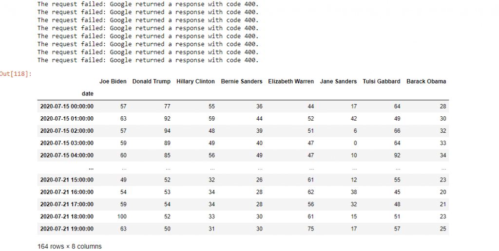
You may see the result above. We have specific 3 days data from the a certain time period. You can also check the graphic below:
How to Check Search Terms’ Interest According to Region by PyTrend
PyTrend also has a special method which is related to the geographic queries.
pytrends.interest_by_region(resolution='COUNTRY', inc_low_vol=True, inc_geo_code=False)- Resolution can be “city”, “country”, “region” according to the targeted area.
- “inc_low_vol” is for including the low volume search data from specific regions.
- “inc_geo_code” is for including the ISO Code of Countries in the data along with their names.
You may see the results for the last three months of search trends for Donald Trump and Joe Biden.
kw_list = [‘Joe Biden’, ‘Donald Trump’]
trendshow.build_payload(kw_list, cat=0, timeframe=’today 3-m’, geo=’US’)
trendshow.interest_by_region(resolution=’COUNTRY’, inc_low_vol=True, inc_geo_code=False)
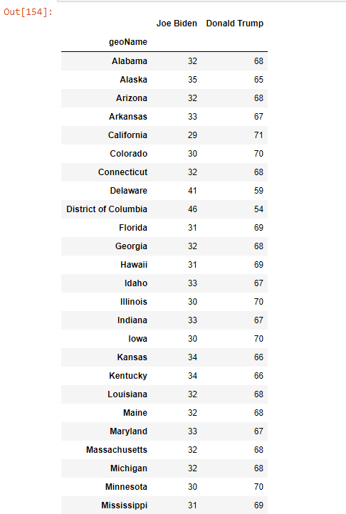
You may also put this into a Map Graphic thanks to Geo-Pandas Library, or you may create a for loop for every different city with subplots.
How to Find Related Searches, Topics and Search Suggestions with PyTrend
Thanks to PyTrend, a Holistic SEO can create his/her own dashboard for a more comprehensive industry and user behavior analysis. The latest trends, search suggestions and related topics for a specific entity can be useful for creating more authority, revenue, traffic and relevance. Content marketing, Brand Language and Communication, Google Ads Campaigns and even the On-Page SEO Elements can be optimized according to the latest and the most relevant search activities.
pytrends.related_topics() method is for finding the most relevant topics for a specific entity. I recommend you to use this for only one query, if you use more than one query, PyTrend will try to find an intersection between queries. And mostly, this process makes no result.
kw_list = [‘Donald Trump’]
trendshow.build_payload(kw_list, cat=0, timeframe=’today 3-m’, geo=’US’)
print(trendshow.related_topics())
The most related topics, entities and their types with Donald Trump is below:
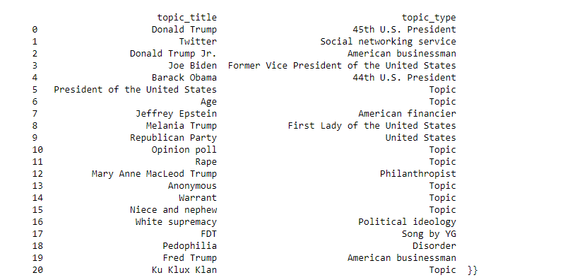
As we can see, related topics consist of entities, not search terms. So, a Holistic SEO can easily see the relationship between entities and their association type via PyTrend. Also, scraping Entity IDs thanks to PyTrend is possible:
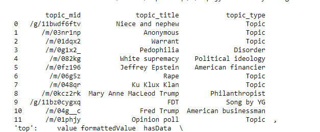
These Entity IDs can help an SEO to use Google’s Knowledge Graph API with Python easier.
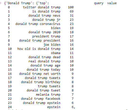
If you wonder the difference between a query and an entity, you need to understand the difference between meaning and string. Now, we will see related strings, instead of entities. The necessary method for this is “related_queries()”.
kw_list = ['Donald Trump']
trendshow.build_payload(kw_list, cat=0, timeframe='today 3-m', geo='US')
trendshow.related_queries()
You may see the most related queries for Donald Trump. Also, you can easily see the difference between an Entity and a Query here. And you may understand why Google needs to understand both of them at the same time. Queries can change the meaning and content of the entities, they can be in an enormous variety and include the smallest details.
Also, you can get the “rising keywords” for a specific query with this method.
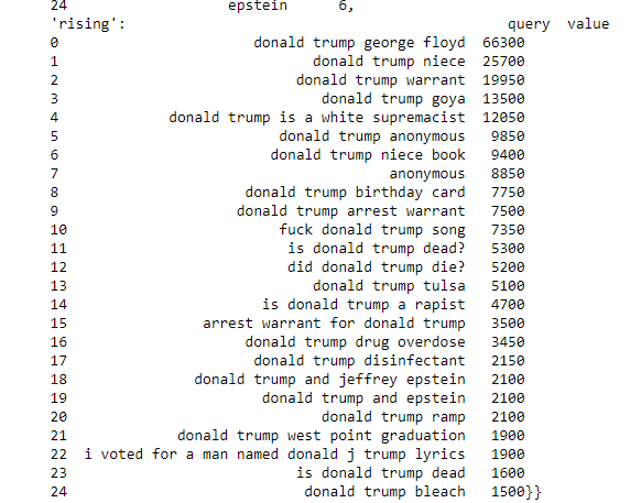
The numbers here can show the increased interest over some queries. For instance, “Donald Trump George Floyd” query is searched more than %66300 in last 3 months for previous timelines. This may help for managing SEO and Google Ads Campaigns in many ways, from understanding the users and optimizing the content and communication.
How to find Trending Searches with PyTrend?
With PyTrend, we may pull the most searched and trending queries for a region. The required method is “trendging_searchers()”.
trendshow.trending_searches(pn='united_kingdom')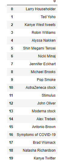
These are the trending searches for United States from 21 July 2020.
How to find suggested topics and queries with PyTrend?
The related method for this is “suggestions(query)”.
dp_df = trendshow.suggestions('donald trump')
dp_df = pd.DataFrame(a)
dp_df
You may see the suggested profiles, searches and features for the query ‘donald trump’. Google gives the entity IDs, entity types for defining the searched query. This data may help a Holistic SEO in his/her content strategy, for a targeted topic and main query, you may need to understand what Google thinks and how Google defines the entity/query. What are the most relevant sides, features and past events for this query? What is the most related other entities? This same process can be done also for “soup”.
sp_df = trendshow.suggestions('soup')
sp_df = pd.DataFrame(sp_df)
sp_df| mid | title | type | |
|---|---|---|---|
| 0 | /m/01z1m1x | Soup | Type of dish |
| 1 | /m/09gms | Ramen | Dish |
| 2 | /m/0ckmp | Chicken soup | Soup |
| 3 | /m/04zwg_ | Lentil soup | Food |
| 4 | /m/03qj953 | Cream of mushroom soup | Food |
If you want to rank yourself in the “soup” query, you may need to include these terms, topics, and related information in a structured way in your content within different formats.
How to pull the most searched trendy queries for a specific month for a country with PyTrend?
The necessary method for this task is the “top_charts()”.
pytrends.top_charts(date, hl='en-US', tz=300, geo='GLOBAL')The date has to be in YYYY or YYYY-MM format like 2017 or 2017-5.
trendshow.top_charts(2020-7, hl='en-US', tz=360, geo='TR')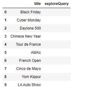
These are the most searched and trendy queries in the US for the 7th months of 2020. I must say that this article is being written on 21st July 2020, it means that this includes only the first 21 days. Also, if you wonder how to pull all the categories in PyTrend, you should use categories() method.
To learn more about Python SEO, you may read the related guidelines to PyTrend Guide:
- How to resize images in bulk with Python
- How to perform TF-IDF Analysis with Python
- How to crawl and analyze a Website via Python
- How to perform text analysis via Python
- How to test a robots.txt file via Python
- How to Compare and Analyze Robots.txt File via Python
- How to Categorize URL Parameters and Queries via Python?
- How to Perform a Content Structure Analysis via Python and Sitemaps
- How to Check Grammar and Language Errors with Python
- How to scrape People Also Ask for Questions from Google via Python
- How to check Status Codes of URLs in a Sitemap via Python
- How to Categorize Queries with Apriori Algorithm and Python
What is the Importance of Search Trends for SEO?
Search Trend Data is one of the most important signals to understand how the mass thinks. It also shows a methodology for analyzing the sentiment related to certain entities. A Holistic SEO can create his/her own Google Trends API thanks to Python and check the search trends along with the organic traffic. If there is a political crisis or pandemic, how people search and behave on the web? If there is a vacation, what people search for? All of these data can be accessed via PyTrend easily and create insight for Holistic SEO.
Also, what is the most related query for an entity? What features do an entity have for specific search intent? Creating a content strategy, understanding the target market, and users’ behavior models during different seasonal and un-ordinary events/situations, managing brand communication, and community management are important pillars for Holistic SEO.
For now, our PyTrend Guideline has tons of missing points. In time, we will refresh and improve it.
- Sliding Window - August 12, 2024
- B2P Marketing: How it Works, Benefits, and Strategies - April 26, 2024
- SEO for Casino Websites: A SEO Case Study for the Bet and Gamble Industry - February 5, 2024



Hello Koray,
Thanks for these codes; these are some excellent information I am learning.
While learning and running the codes, I found two or three errors, some due to the inverted commas. When I copy-pasted, it gave a different inverted comma, because of which the error is happening.
kw_list = [‘Joe Biden’, ‘Donald Trump’]
trendshow.build_payload(kw_list, cat=0, timeframe=’today 3-m’, geo=’US’)
It should be…
kw_list = [‘Joe Biden’, ‘Donald Trump’]
trendshow.build_payload(kw_list, cat=0, timeframe=’today 3-m’, geo=’US’)
Also, for one more error was ..
dp_df = trendshow.suggestions(‘donald trump’)
dp_df = pd.DataFrame(a)
dp_df
The code should be
a = trendshow.suggestions(‘donald trump’)
dp_df = pd.DataFrame(a)
dp_df
I used to check google trends by inserting individual keywords, and now, this is very easy.
Thanks again for your help brother.
Regards
Madhan